How to Forecast Silver Prices With NeuralProphet And Python

Is it possible to forecast silver prices with Python? Yes, and in this tutorial, I will show you how I do it using NeuralProphet and Python. If you want to just grab all the code right away, just navigate down to the Silver Prices Forecasting NeuralProphet Model Code section.
Before we begin, we need to make sure we have all the right Python libraries loaded into our environment. Aside from the standard matplotlib, pandas, and numpy libraries, you will need to install yfinance and neuralprophet.
import pandas as pd
from pandas import to_datetime
import matplotlib.pyplot as plt
import numpy as np

import yfinance as yf

from neuralprophet import NeuralProphet, set_log_level
Once you've installed these libraries you can start writing a few data and ETL functions, most notably where to pull silver prices and how to calculate a rolling volatility calculation.
Silver Prices Extraction
I like to write functions to make my life easier and the first one I have in the code is getting the silver prices from yfinance. It's pretty simple and for this example, I wanted to download 240 months of silver prices.
You can change the period to anything you like, at the minimum I would recommend at least 12 months of data.
def get_ticker_data(tckr):
    tmp = yf.Ticker(tckr)
    df = tmp.history(period="240mo")
    return df
Silver Prices Volatility
The next function I use is to calculate a rolling volatility for silver prices. I do this because I want to add the volatility as a lagged regressor in the NeuralProphet model.
def volatility_calc(df):
    df['Volatility'] = (df['High']-df['Low']).rolling(4).std()*(52**0.5)
    df['Volatility Pct Change'] = df['Volatility'].pct_change()
    return df
The volatility calculation is pretty simple, just get the daily price range (high - low) over a 4-day period. I calculate both the raw volatility value and the percent change, then return it as two new columns in my data frame.
Load Silver Prices Data
Now we invoke the functions and save the results as a data frame df.
out = get_ticker_data('SI=F')
df = volatility_calc(out)
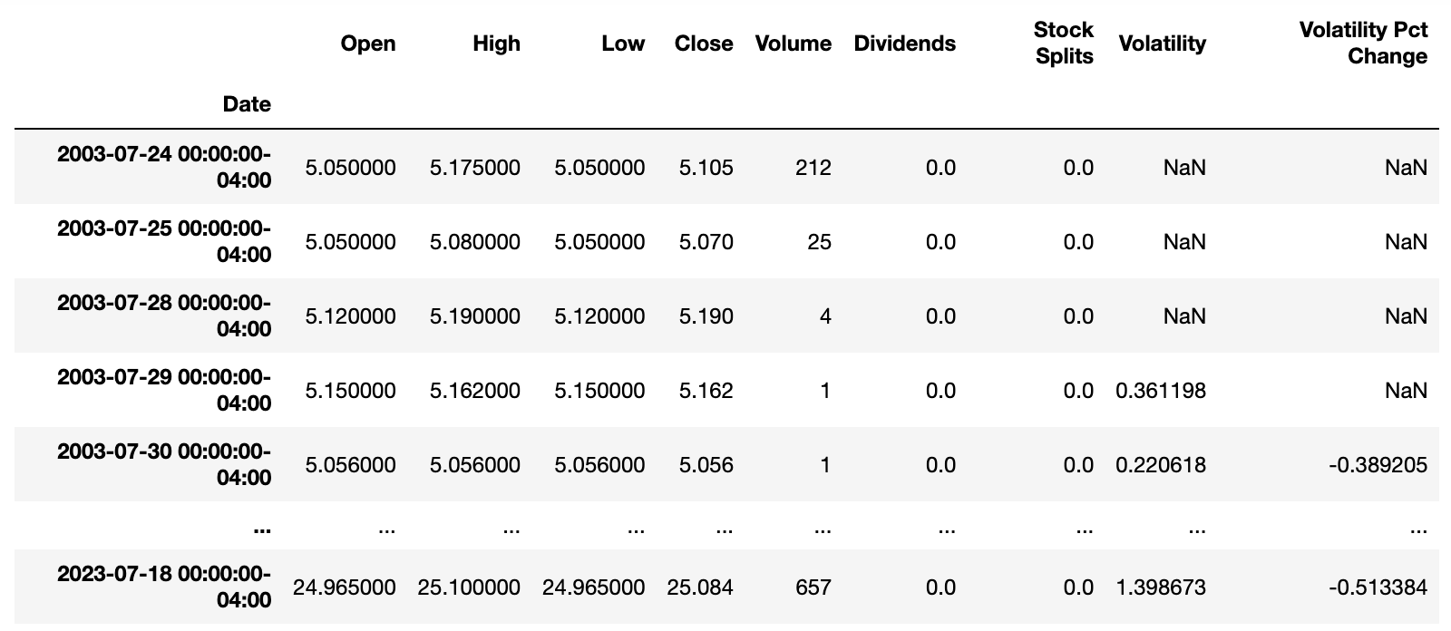
NeuralProphet requires that we shape the data in a specific way so that it can do its analysis. We need to feed in the data with at least two columns that are labeled (or named) as ds and y, our date stamp, and our series value respectively.
Since we're adding a third column, an additional regressor called Volatility we have to make sure that it's the final dataframe as well. So we first drop all columns except for the Date Index, Close, and Volatility.
We reset_index() the Date Index to a date, make sure it's parsable as a date time, and rename it to the ds. We also renamed the Close column to y and left Volatility along.
df = df[['Close','Volatility']]
df = df.reset_index()
df['Date'] = pd.to_datetime(df['Date'])

df = df[['Date', 'Close','Volatility']]
df = df.rename(columns={"Date": "ds", "Close": "y"})
df['ds'] = df['ds'].dt.tz_localize(None)
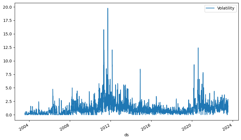
For fun we plot the y series over time and we do the same for the Volatility series too. Note, I didn't add a title or any other labeling, just the ones that came out of the box.
plt = df.plot(x="ds", y=["y"], figsize=(10, 6))
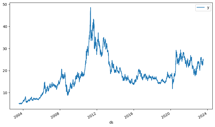
These plotting steps are just intermediary, done so I can make sure I'm not messing anything up.
plt = df.plot(x="ds", y=["Volatility"], figsize=(10, 6))
The NeuralProphet Silver Prices Forecast Model
NeuralProphet is such a wonderful time series forecasting package. It was inspired by Facebook Prophet and AR-Net, built on Pytorch,, and let's you do standard time series modeling like FBProphet or use autoregressive features that automatically detrend your forecasts like ARIMA.
You're going to have to make a choice if you want to do an autoregressive model or the standard time series modeling. You will get different results with one method having better performance, so you will need to check.
I defined my silver prices forecasting model as one that's autoregressive, it will automatically detrend the time series but it will only give me a one period lookahead prediction. Conversely, my FBProphet forecasting model is a standard time series one where I forecast 1 to 5 (or more) periods ahead.
The one period time forecast is really the freq parameter below and it can be set as auto, D,W, or M. If you just auto it will use the time period that your time series is already set at in the data.
m = NeuralProphet(
    growth="off",
    yearly_seasonality="auto",
    weekly_seasonality="auto",
    daily_seasonality="auto",
    n_lags=10,
    num_hidden_layers=20,
    d_hidden=36,
    learning_rate=0.003,
    n_forecasts = 1,
    n_changepoints = 3,
    changepoints_range=0.95,
)

m.add_lagged_regressor("Volatility")
metrics = m.fit(df, freq='auto')
A lot of the model is set at auto and NeuralProphet handles a lot of the time conversions automatically, as well as the hyperparameter tuning. It's quite nice in that sense.
For this particular model, I turned on the autoregressive feature by using the growth parameter, even if it's set to off by calling this parameter I told NeuralProphet that I want to use autogression.
I wanted to know if my data had daily, weekly, or yearly seasonality so I set those parameters to auto as well.
Next, I defined how many lags my autogression should have by setting a value of 10 for n_lags.
Then I defined how I want my neural network to look by setting num_hidden_layers=20, d_hidden=36, and learning_rate=0.003.
Finally, I tell NeuralProphet how many forecasts into the future I want via n_forecasts=1 and I give it some options for how many trend change points I have over the time series via the n_changepoints = 3, and changepoints_range=0.95 parameters.
There are many more parameters you can use, just check out the documentation for NeuralProphet and NeuralProphet hyperparameter tuning.
The last thing we have to do is add the Volatility regressor and invoke the model to train our silver prices forecast. To do that we add m.add_lagged_regressor("Volatility") and then train the model with metrics = m.fit(df, freq='auto').
Note, the freq parameter can be set to auto, or D or W, or whatever time period you want. NeuralProphet will handle the resampling and conversion if you have a daily (D) time series to weekly (W) if you set the freq parameter to W.
Evaluating the Silver Prices Forecast Model
Invoke and run the model and then calculate the losses. This is important because you want to know just how well the model is predicting vs. the actual silver prices.
A word of caution, forecasting silver prices or any other financial asset is hard, sometimes impossible. There are so many moving parts to these markets that one bit of bad news could send prices in the opposite direction.
metrics.tail(1)

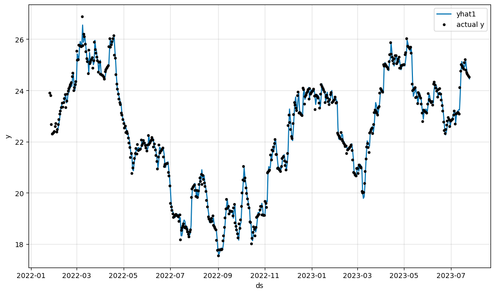
Next, we calculate our forecasts and plot the actual silver prices versus the predicted ones using the following code.
df_future = m.make_future_dataframe(df, n_historic_predictions=365, periods=1)

forecast = m.predict(df_future)
fig = m.plot(forecast)
Our resulting plot looks like this below:
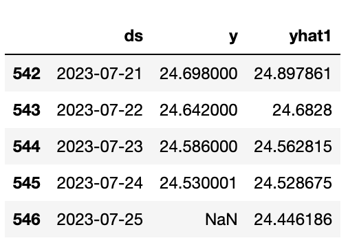
If you want to get the actual value that's forecast one day ahead, just run.
forecast[['ds','y', 'yhat1']].tail()
Silver Prices Forecast Model and Parameter Components
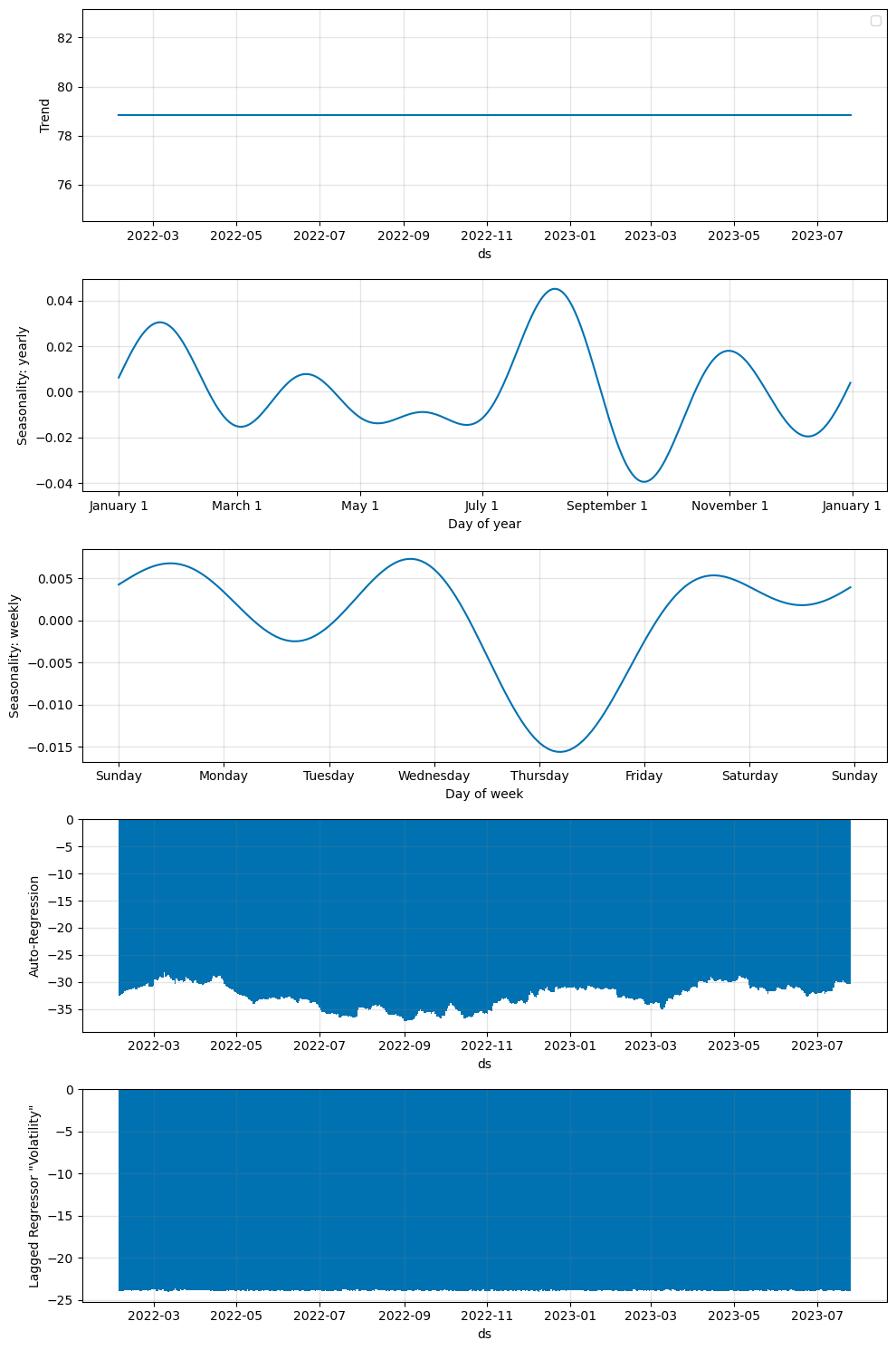
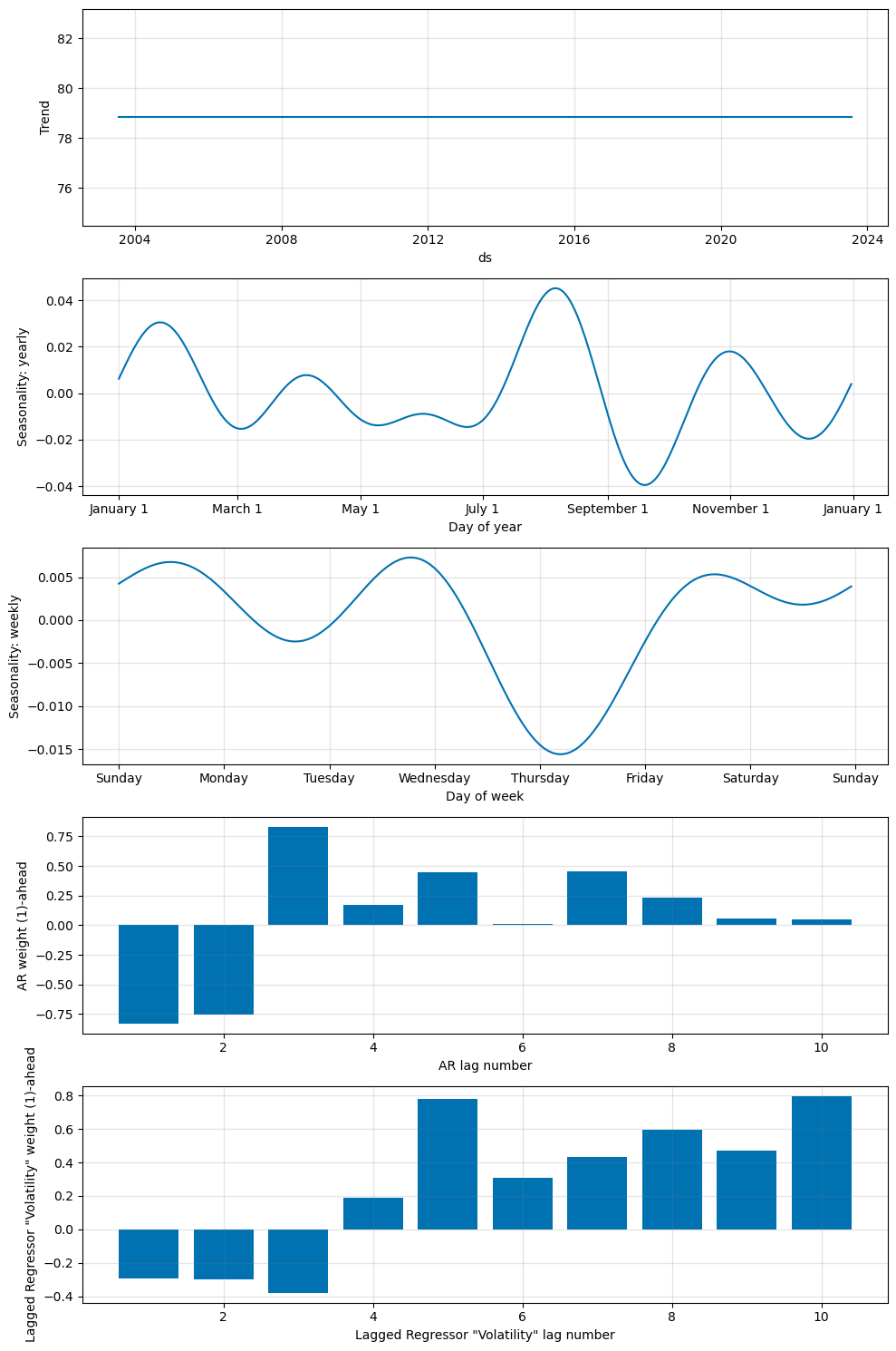
Sometimes you need to see the NeuralProphet model components and parameters for things like trend (or no trend in our case) or seasonality. To do that you invoke fig_comp = m.plot_components(forecast) to get the model components and fig_param = m.plot_parameters().
You'll get the following plots generated:
Plot Silver Prices Forecast Residuals
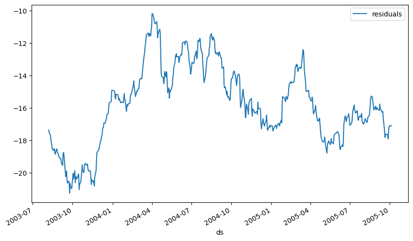
The last thing we want to do is check out far off our predictions were from the true value. For that, we need to make a residual plot of the true values from the prediction.
Generating a residual plot in NeuralProphet is as simple as doing this:
df_residuals = pd.DataFrame({"ds": df["ds"], "residuals": df["y"] - forecast["yhat1"]})
fig = df_residuals.plot(x="ds", y="residuals", figsize=(10, 6))
When you do that you get this nice chart and you can evaluate how stable your model is.
The Entire Silver Prices Forecasting NeuralProphet Model Code
When you pull all these pieces together into one Python script, you get the following full code.
import pandas as pd
from pandas import to_datetime
import matplotlib.pyplot as plt
import numpy as np

import yfinance as yf

from neuralprophet import NeuralProphet, set_log_level

def get_ticker_data(tckr):
    tmp = yf.Ticker(tckr)
    df = tmp.history(period="240mo")
    return df

def volatility_calc(df):
    df['Volatility'] = (df['High']-df['Low']).rolling(4).std()*(52**0.5)
    df['Volatility Pct Change'] = df['Volatility'].pct_change()
    return df

out = get_ticker_data('SI=F')
df = volatility_calc(out)

df = df[['Close','Volatility']]
df = df.reset_index()
df['Date'] = pd.to_datetime(df['Date'])

df = df[['Date', 'Close','Volatility']]
df = df.rename(columns={"Date": "ds", "Close": "y"})
df['ds'] = df['ds'].dt.tz_localize(None)

plt = df.plot(x="ds", y=["y"], figsize=(10, 6))

plt = df.plot(x="ds", y=["Volatility"], figsize=(10, 6))

m = NeuralProphet(
    growth="off",
    yearly_seasonality="auto",
    weekly_seasonality="auto",
    daily_seasonality="auto",
    n_lags=10,
    num_hidden_layers=20,
    d_hidden=36,
    learning_rate=0.003,
    n_forecasts = 1,
    n_changepoints = 3,
    changepoints_range=0.95,
)

m.add_lagged_regressor("Volatility")
metrics = m.fit(df, freq='auto')

metrics.tail(1)

df_future = m.make_future_dataframe(df, n_historic_predictions=365, periods=1)

forecast = m.predict(df_future)
fig = m.plot(forecast)

forecast[['ds','y', 'yhat1']].tail()

fig_comp = m.plot_components(forecast)

fig_param = m.plot_parameters()

df_residuals = pd.DataFrame({"ds": df["ds"], "residuals": df["y"] - forecast["yhat1"]})
fig = df_residuals.plot(x="ds", y="residuals", figsize=(10, 6))
End Notes
This tutorial is what I used in the early days of my silver prices forecasting project. I created this model as a way to help me figure out what silver prices were going to do in the immediate future because I'm a coin collector.
I wanted to forecast where silver prices and volatility were headed and know if I had to pay more for a premium or spread when buying American Silver Eagles or Junk Silver coins.
This model has undergone many evolutions as I added more regressors and different features into the model to make my forecasting more robust. As I cautioned before, these forecasts can be very volatile and turn quickly wrong if a wild news event happens. That's the nature of the market.
Drop me a comment if you have questions.


Member discussion